Back to Notes

Example 1

Consider the autonomous equation

\[y' = f(y) = (9y+1)(y-5)(y+3)^2.\]

We see that $f(c) = 0$ only for the values $c = 5, -3, -1/9$. These correspond the equilibrium solutions $y(t) = 5$, $y(t) = -3$ and $y(t) = -1/9$ to the differential equation.

In order to figure out the behavior of solutions $y$, we need to know the behavior of the function $f(y)$ for $y<-3$, -3<y<-1/9$, $-1/9<y<5$ and $y>5$. We now compute the signs of $f$ on these regions:

\[\begin{split} f(-10) &= (-)(-)(+)>0\\ f(-1)&= (-)(-)(+)>0\\ f(0) &= (+)(-)(+)<0\\ f(10) &= (+)(+)(+) >0. \end{split}\]

Therefore, we know the graph of $f$ should look something like:

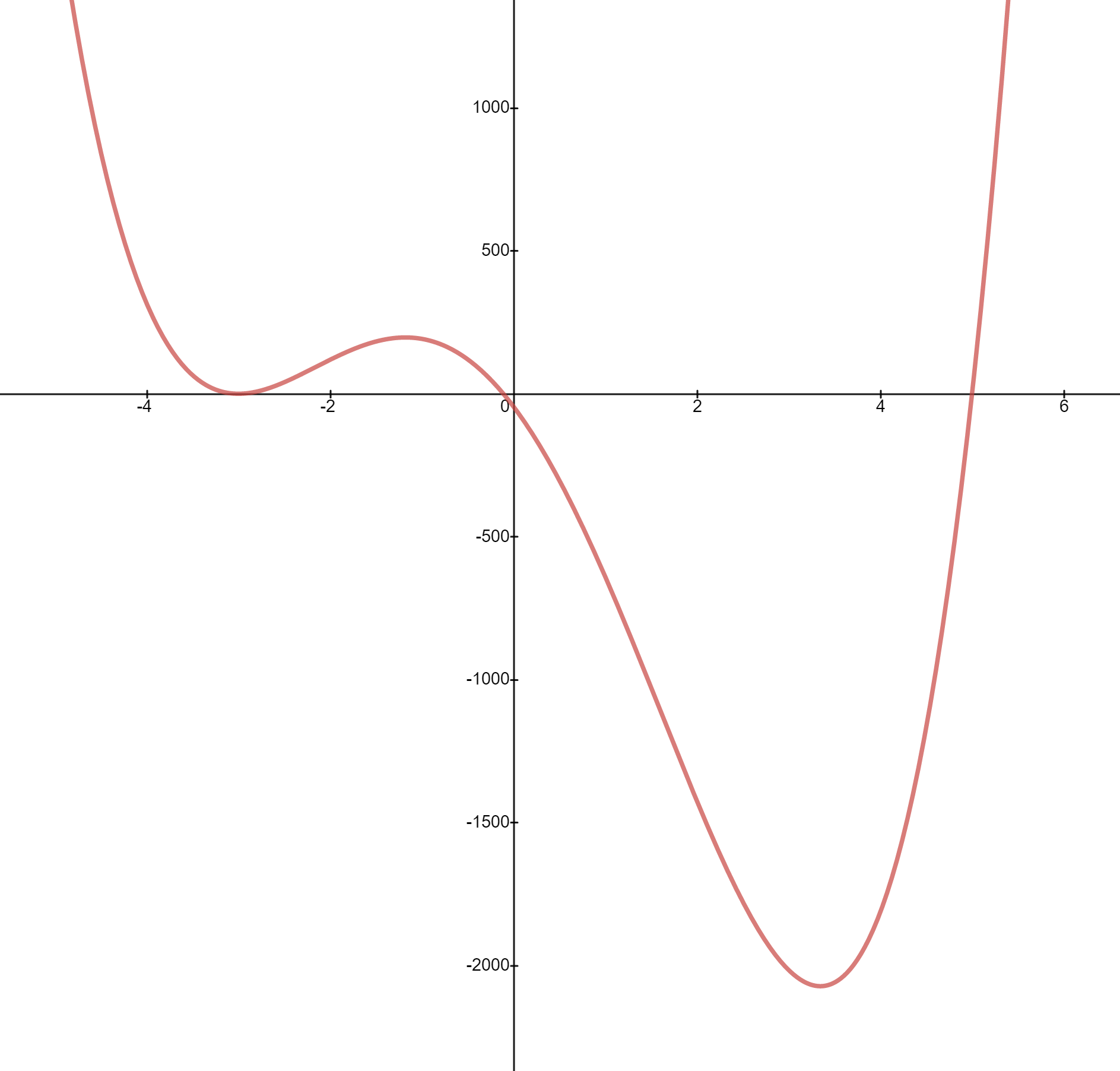
The above picture is an actual graph of $f(y)$ in red with $y$ in the horizontal axis. We can also write the phase diagram:

From this picture (well even from the graph of $f$ above) we see that

• The solution $y=-3$ is semistable
• The solution $y=-1/9$ is stable
• The solution $y = 5$ is unstable

Here is a picture of some (approximations of) solutions:

where the blue ($y=5$), green $(y=-1/9$) and red ($y=-3$) are the equilibrium solutions. I don’t have the time (horizontal) axis labelled because this is operating on a very small time scale (about $0\le t\le 1/1000$).

What else can we answer? Let

\[\begin{split} L(y_0) &= \lim_{t\to\infty} y(t),\\\ \text{when }\qquad y' &= f(y) ,\quad \text{and}\quad y(0) = y_0. \end{split}\]

We allow the case $L(y_0) = \pm \infty$.

Then we see

• When $y_0 > 5$, the solutions increase without bound and so $L(y_0) = \infty$;
• When $-1/9<y_0<5$ the solutions decrease, but cannot cross the equilibrium solution $y = -1/9$ and so $L(y_0) = -1/9$;
• When $-3<y_0 < -1/9$ the solutions increase, but cannot cross the equilibrium solution $y = -1/9$ and so $L(y_0) = -1/9$;
• When $y_0<-3$ the solutions increase, but cannot cross the equilibrium solution $y= -3$ and so $L(y_0) = -3$.

Example 2

Consider

\[y' = f(y) = y(y+1)^2(y-5)(y+6)^2.\]

The roots of $f$ and the equilibrium solutions are

\[0, -1, 5, -6.\]

Doing a similar computations as in example 1, we can see that the graph of $f$ should look like the picture below (I actually just plotted the actual graph):

The graph of $f$ is massive in some areas and small in some areas as well. By that I mean we had to cut off the graph near $f(y)<-2500$ in order to continue to see what happens between $-1$ and $0$. This big disparity between the magnitude of $f(y)$ will affect quantitative properties of solutions, by which I mean if we drew the slope field and the solutions as in Example 1, some solutions would look very flat.

But from here we can draw the phase diagram:

Neglecting my poor handwriting, from here we can see the following stability:

• 5 is unstable
• 0 is stable
• -1 and -6 are semistable.

The limits can be computed as well

\[\begin{split}L(y_0) &= \lim_{t\to\infty} y(t),\\ \text{when }\qquad y' &= f(y) ,\quad \text{and}\quad y(0) = y_0.\end{split}\]

• When $y_0>5$, the limit is $\infty$
• When $0<y_0<5$ the limit is $0$
• When $-1<y_0<0$ the limit is $0$
• When $-6<y_0<-1$ the limit is $-1$
• When $y_0<-6$ the limit is $-6$.