Example 1
Let us start with a simple example:
\[\text{Estimate }y(5)\text{ when }y\text{ solves } \left\{ \begin{array}{l} y' = t\\ y(0) = 0 \end{array} \right.,\quad \text{with }\, \Delta t = 1.\]Now by the fundamental theorem of calculus, if $y’ =t$ and$y(0) = 0$ then
\[y(t) = y(t) - y(0) = \int_0^ty'(t)\,dt = \int_0^t t\,dt = \frac{1}{2}t^2.\]Let us try to approximate $y(5)$ using Euler’s method.
We start with
\[y(1) \approx y(0) + y'(0)\Delta t = 0 + 0 \times 1 = 0.\]We then try to approximate $y(2)$ from that above estimate of $y(1)$:
\[y(2) \approx y(1) + y'(1)\Delta t \approx 0 + 1\times 1 = 1.\]Continuing on this way we get the following
\[\begin{array}{l} y(3) \approx y(2)+y'(2)\Delta t \approx 1+ 2\times 1 =3\\ y(4) \approx y(3)+y'(3) \Delta t \approx 3+3\times 1 = 6\\ y(5) \approx y(4) + y'(4) \Delta t \approx 6+4\times 1 = 10. \end{array}\]Which gives an approximation of $y(5)$ as $10$. However, we know that the real value of $y(5) = \frac{1}{2}(5)^2 = 12.5$.
We can write the information computed above in the following table, which is often much easier to deal with then a bunch of equations as above:
| $n$ | $y_n\approx y(t_n)$ | $t_n$ | $\Delta t$ | $y’_n \approx y’(t_n)$ | $y_{n+1}\approx y(t_n+\Delta t)$ |
|---|---|---|---|---|---|
| 0 | 0 | 0 | 1 | 0 | 0 |
| 1 | 0 | 1 | 1 | 1 | 1 |
| 2 | 1 | 2 | 1 | 2 | 3 |
| 3 | 3 | 3 | 1 | 3 | 6 |
| 4 | 6 | 4 | 1 | 4 | 10 |
We always write $t_n - t_{n-1} = \Delta t$. We stop after step $n = 4$ because the last term is the approximation of $y(4+1) = y(5)$.
The error can be seen with the following image:
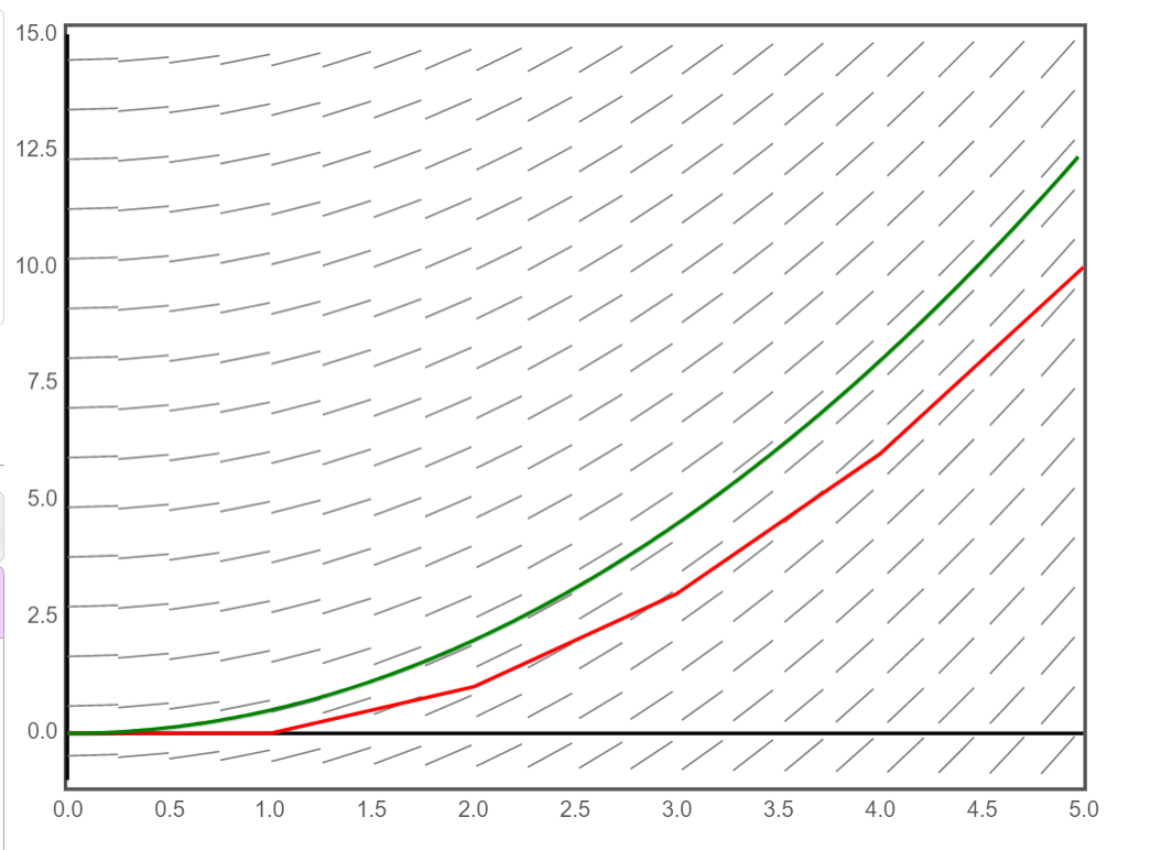
Above the red line is the approximation from Euler’s method (with straight lines drawn between the points computed above) and the green line is the actual solution.
If we instead set $\Delta t = 0.5$ then we get the following information:
| $n$ | $y_n \approx y(t_n)$ | $t_n$ | $\Delta t$ | $y’_n \approx y’(t_n)$ | $y_{n+1} \approx y(t_n+\Delta t)$ |
|---|---|---|---|---|---|
| 0 | 0 | 0 | 0.5 | 0 | 0 |
| 1 | 0 | 0.5 | 0.5 | 0.5 | 0.25 |
| 2 | 0.25 | 1 | 0.5 | 1 | 0.75 |
| 3 | 0.75 | 1.5 | 0.5 | 1.5 | 1.5 |
| 4 | 1.5 | 2 | 0.5 | 2 | 2.5 |
| 5 | 2.5 | 2.5 | 0.5 | 2.5 | 3.75 |
| 6 | 3.75 | 3 | 0.5 | 3 | 5.25 |
| 7 | 5.25 | 3.5 | 0.5 | 3.5 | 7 |
| 8 | 7 | 4 | 0.5 | 4 | 9 |
| 9 | 9 | 4.5 | 0.5 | 4.5 | 11.25 |
We stop after step 9 above because the last term in the table (the bottom right) is the approximation of $y(4.5+\Delta t) = y(5)$. As you can tell $11.25$ is closer to the actual value of $y(5)$ than $10$.
Here is the associated graphical depiction of what the above table does.

Example 2
Let us consider the following more complicated example:
\[\text{Estimate } y(1) \text{ when }y \text{ solves } \left\{ \begin{array}{l} y' = \displaystyle\frac{t^2}{3} + 6 + \frac{y}{4}\\ y(0) = 5 \end{array} \right.\qquad \text{with}\quad \Delta t = 0.2\]I’ll just include a table with all the important information with approximations rounded to two decimal places:
| $n$ | $y_n \approx y(t_n)$ | $t_n$ | $\Delta t$ | $y’_n \approx y’(t_n)$ | $y_{n+1}\approx y(t_{n}+\Delta t)$ |
|---|---|---|---|---|---|
| 0 | 5.00 | 0 | 0.2 | 7.25 | 6.45 |
| 1 | 6.45 | 0.2 | 0.2 | 7.63 | 7.98 |
| 2 | 7.98 | 0.4 | 0.2 | 8.07 | 9.59 |
| 3 | 9.59 | 0.6 | 0.2 | 8.58 | 11.31 |
| 4 | 11.31 | 0.8 | 0.2 | 9.15 | 13.14 |
Here’s the image:
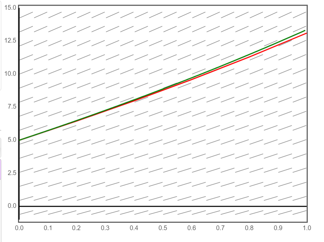
As you can see, the red solution is very close to the actual solution (shown in green). This is partly because we chose $\Delta t = 0.2$ which is fairly small. It is also, in part, due to the particular differential equation we worked with.